Delayed Tensor Parallelism for Faster Transformer Inference
DTP is a new Transformer architecture that hides communication overhead behind computation and weight streaming, enabling significantly faster batch-size-one inference on AMD and NVIDIA GPUs.

Modern LLM inference is increasingly shaped by latency-critical workloads: multi-step agentic workflows, real-time copilots, voice assistants, and reasoning systems that generate long chains of thought. In these settings, batch-size-one token generation speed, not aggregated throughput, is the metric that matters. But in this setting, decoding latency becomes dominated by memory movement and synchronization overhead rather than raw compute.
In this post, we introduce Delayed Tensor Parallelism (DTP), a new architecture designed to hide communication behind computation and weight streaming. We show that DTP preserves the quality of standard tensor-parallel Transformer architectures while dramatically reducing exposed communication costs, enabling much faster inference on modern AMD and NVIDIA GPUs.
Introduction
LLMs are typically optimized for throughput: serving many users at once with large batch sizes to maximize hardware utilization. But not all applications live in that regime.
Typically for applications such as voice assistants, real-time copilots, reasoning models and agentic workflows, what matters for users is latency at batch size one. In this regime, the bottlenecks shift: performance is no longer compute-bound, but dominated by weight streaming, kernel launch overheads, and memory movement.
A natural way to reduce these costs is to shard the model across multiple GPU devices. In practice, this is done with Tensor Parallelism [1] (TP), which splits the computation of attention and MLP layers across GPUs.
But TP is not a free lunch. It introduces communication overhead that can wipe out its benefits. This becomes especially painful when every other bottleneck such as weight streaming continuity and kernel granularity are already super-optimized [Monokernel].
A fairly natural way to alleviate this communication overhead is simply to parallelize the model in the way TP does while completely removing communications. However, we show that training from scratch with such no-communication architecture variant heavily degrades performance.
To claw back the performance gap introduced by communication removal, the Kog Team proposes Delayed Tensor Parallelism (DTP). DTP is an architectural variant of the base Transformer model that allows the TP scheme to overlap communication and computation. As a result, training a LLM with the DTP architecture gets the best of both worlds, meaning that it alleviates communication overhead while keeping performance in the same ballpark.
We show the former points experimentally: pretraining with our architecture variant instead of the usual Transformer blocks claws back quality w.r.t to the version without communication. In fact, performance-wise, DTP stands very close to the vanilla Transformer blocks.
Furthermore, in our batch-size one target setup, we compare DTP with state-of-the-art methods for communication overhead reduction and we show that, when aiming at no communication overhead, DTP can significantly outperform them.
Strong with those findings we pretrained a 2B-parameter model with DTP. This model includes all Kog's GPU team optimizations plus our DTP innovative architecture and achieves unprecedented speed on AMD and NVIDIA datacenter GPUs.
Background on Tensor Parallelism
Tensor Parallelism [1] (TP) is usually the go-to technique when sharding a Transformer architecture across several GPU devices, especially when the model at hand fits into the aggregated memory of the GPUs on a single node.
In TP, weights are sharded across devices on a per-module basis, where a module refers to either an MLP or attention block. For a given module, each device performs its partial forward pass using its local parameter shard, then the partial outputs are aggregated via an all-reduce operation to recover the result equivalent to single-device execution.
More formally, for a Transformer with hidden size \(d\), let \(\mathbf{X}^{(n)} \in \mathbb{R}^{S \times d}\) denote an input of sequence length \(S\) to the \(n\)-th Transformer module \(\mathbf{M}^{(n)}(\cdot\,; \theta)\) with parameters \(\theta\). Under TP with \(L\) devices, the parameter set is partitioned into disjoint shards \(\theta_l\), and the module output is computed as:
\[\mathbf{X}^{(n+1)} = \mathbf{X}^{(n)} + \sum_{l=1}^{L} \mathbf{o}_l^{(n)},\]where each term \(\mathbf{o}_l^{(n)} = \mathbf{M}^{(n)}(\mathbf{X}^{(n)};\theta^{(n)}_l)\) is the local output of module \(n\) computed on device \(l\). Figure 1 summarizes the computational graph of a TP layer.
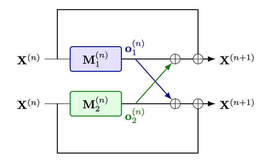
By enabling parallel streaming of parameter shards, TP can significantly reduce inference latency in memory-bound settings. However, it introduces a synchronization cost: each Transformer module requires an all-reduce operation to ensure equivalence with the non-partitioned model. This communication overhead can become a critical bottleneck.
These observations motivate approaches that overlap communication with computation to mitigate synchronization overhead. In this spirit, we introduce delayed communications strategies that hide all-reduce latency behind subsequent computations, thereby improving end-to-end inference efficiency.
Delayed Tensor Parallelism (DTP)
The core idea of DTP is to overlap TP communications with concurrent computation or weight streaming. In that spirit, we propose to delay this all-reduce operation across modules: at the end of a module we launch the communication of each device local output to all other devices, though we do not all-reduce those outputs straight away as TP would. Instead we proceed to the computation of the \(\delta\) next modules based on the local outputs. At the end of those \(\delta\) modules we reduce current outputs from each device with the outputs from \(\delta\) modules in the past. By doing that, we provide enough time for communications from each device to land on the other devices. Naturally, this strategy splits the model computational graph into 3 stages:
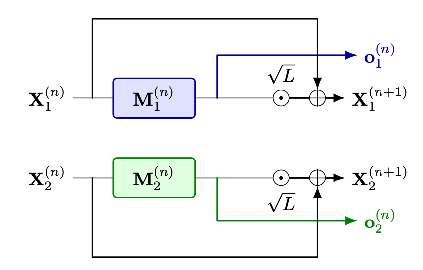
First, for the \(\delta\) first layers, nothing is aggregated from the past layers. The local output of each device is simply sent to all other devices and then used locally for computation of the next module. Formally for the input \(\mathbf{X}_l^{(n)}\) for device \(l\) and layer \(n < \delta\), the input to the next module is computed as follows:
\[\mathbf{X}_l^{(n+1)} = \mathbf{X}_l^{(n)} + \sqrt{L}\, \mathbf{o}_l^{(n)}\]where the \(\sqrt{L}\) factor is designed to mimic the scale of the all-reduce communication. Contrary to TP, local output for device l at layer n depends on local input for device l : \(\mathbf{o}_l^{(n)} = \mathbf{M}^{(n)}(\mathbf{X}^{(n)}_l;\theta^{(n)}_l)\)
Second, for the n-th module with \(n \in [\delta, 2N_L - \delta]\) where \(N_L\) is the number of layers, local module outputs are sent to the network and the past module outputs are aggregated with the local output to form the input to the next module:
\[\mathbf{X}_l^{(n+1)} = \mathbf{X}_l^{(n)} + \mathbf{o}_l^{(n)} + \sum_{j \neq l} \mathbf{o}_j^{(n-\delta)}\]where \(\mathbf{o}_l^{(n)}\) is the local output of device l and \(\sum_{j \neq l} \mathbf{o}_j^{(n-\delta)}\) is the sum of local outputs from past modules.
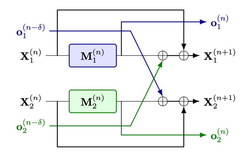
Finally for the \(\delta\) last modules, no communication with other devices is required and the past is aggregated as in the steady-state equation above.
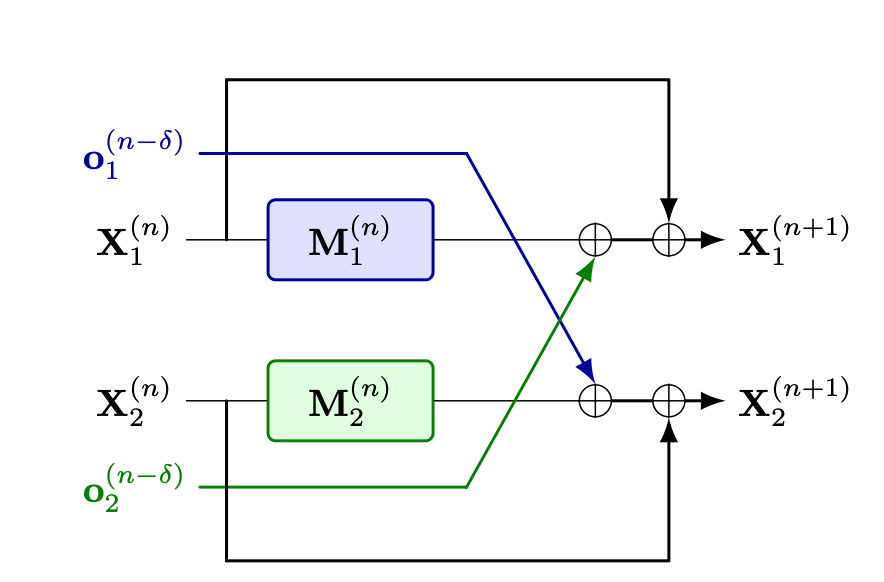
At the end of the \(2N_L\) modules, a final layernorm along with the LM-head of size \(d \times V\), where \(V\) is the size of the vocabulary, is applied to each device local output and the \(L\) outputs are averaged in a final all-reduce operation.
Experiments
Implementation Details
All our experiments are based on the Llama3 architecture that is implemented in torchtitan with vocabulary size \(V = 32000\). We mostly experimented with two different architectural setups that are reported in Table 1. As far as the training dataset is concerned we use the Climbmix dataset [2] with sequence length \(S = 1024\). From an optimization point of view we use batch-size = 512 and we train to reach 20 tokens per parameter with a learning rate that follows a WSD schedule with 250 warm-up steps to reach a steady-state value of \(lr = 5 \times 10^{-4}\) and then a decay phase of 10% of the total training steps.
| Identifier | \(N_L\) | \(d\) | \(n_h\) | Size | Steps | LR |
|---|---|---|---|---|---|---|
| Architecture 1 (A1) | 24 | 1024 | 16 | 367M | 14,081 | \(5 \times 10^{-4}\) |
| Architecture 2 (A2) | 16 | 1536 | 24 | 551M | 21,031 | \(5 \times 10^{-4}\) |
Preliminary Experiments
The most naive way to alleviate the TP communication overhead is to remove synchronized communications. Typically at the end of a module, we do not send local latents to other devices but simply forward them to the next module.
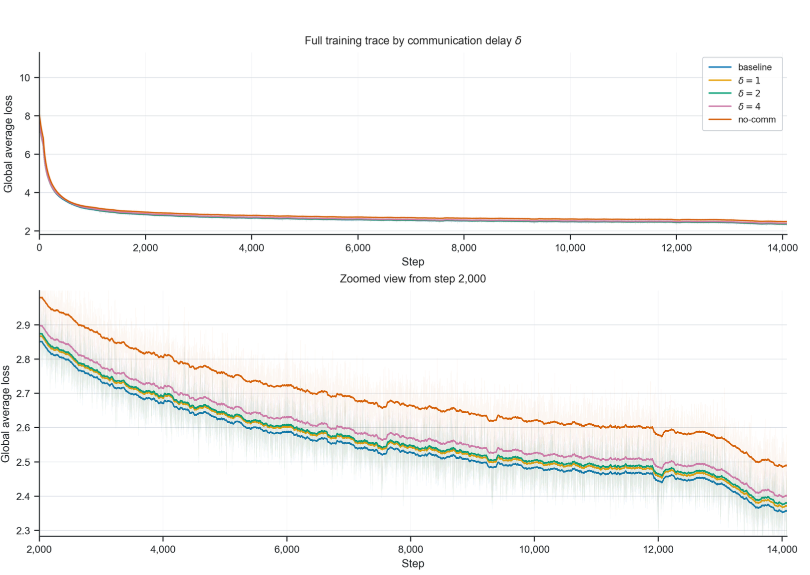
Figure 5 shows a training loss comparison between (a) the Llama baseline which uses fully synchronized communications at the end of all modules (b) the version without any communication (no-comm) (c) our DTP variant with different values for the broadcast delay \(\delta\). We clearly observe that completely removing the communication from the TP scheme significantly degrades training performance. On the other side, we observe that DTP claws back most of the performance loss. Naturally as delay \(\delta\) increases, we observe that performance slowly drops in the direction of the no-communication version. Yet even with delay \(\delta = 4\) which in our setup allows us to hide all TP communications while remaining close to the fully synchronized baseline.
Comparison with SOTA methods
In this section we compare the DTP method with existing methods to reduce or cache communication overhead at inference time, namely:
- GPT-J [3]: A modification of the Transformer architecture that parallelizes MLP and Attention modules hence reducing the need for all-reduce synchronization from 2 to 1 per layer.
- Ladder-Residual [4]: A modification of the Transformer architecture that uses the residual of a module as input to the next module, similar to our method, allowing to hide communication behind computation. Typically, at the end of the computation of the n-th attention, the computation of the n-th MLP can be launched from the residual without having to wait for the attention all-reduce to finish.
- PT-Transformer [5]: Similar to what we did with the no-comm version of Llama3, PT-Transformer removes all-reduce synchronization for all Attention modules and keeps it only for 1 out of \(t_d\) MLP.
We also tried to compare with Kraken [6]. However, the caveat of Kraken is that it modifies the size of the decoder so that we cannot get comparisons at exact same size. In fact what we tried to do was get the closest candidates in size (one candidate with a slightly lower parameter count and one with a slightly higher parameter count). However, with that methodology even the candidate with the higher parameter count gave poor results. More precisely, in that setup, DTP and all other communication overhead reduction methods outperformed Kraken by a wide margin.
Theoretical Exposed Wait-time
In the batch-size 1 setup that we are targeting, inference is memory-bound. That means that the bottleneck is not the speed at which operations are computed (FLOPs) but rather the speed at which weights are loaded from High Bandwidth Memory (HBM) to Compute Units (CU) or Streaming Multiprocessors (SM).
Consequently, to determine which of those methods is most adapted to our setting we place ourselves in an ideal setup in which (a) weight streaming is the bottleneck (b) model weights are streamed continuously from the HBM to the CUs/SMs. To measure the efficiency of the different methods at reducing communication overhead, we define the theoretical exposed wait-time as the communication time that cannot be hidden by weight-streaming.
- Baseline: For the full-comm baseline, each Transformer block requires an all-reduce communication. Hence the exposed wait-time is \(\Delta_B = 2N_L \tau_c\) where \(\tau_c\) is the communication latency.
- GPT-J: Since MLP and Attention are computed in parallel, only a single all-reduce is required at the end of each Transformer block. Exposed wait-time is therefore \(\Delta_J = N_L \tau_c{.}\)
- PT-Transformer: In PT-Transformer, attention all-reduces are removed and only 1 out of \(t_d\) all-reduces is kept for the MLP, hence an exposed wait-time of \(\Delta_J = N_L\tau_c.\)
- Ladder Residual: Ladder Residual allows caching of communication behind weight streaming by using the output of the residual of the n-th module as input to module n + 1. Computing theoretical exposed wait-time is therefore slightly more complicated. Typically if we look at it module-wise, to start the weight streaming for module n + 1 we need the output of module n − 1 that is an all-reduce communication. Though instead of waiting for the all-reduce, we can stream module n. Hence, some wait-time gets exposed if streaming module n takes less time than \(\tau_c\). In formal terms, exposed wait-time for module \(n \in [2, 2N_L - 1]\) is \(\max(0, \tau_c - \tau_w^{(n-1)})\), where \(\tau_w^{(n)}\) is the time taken to stream module n. There remain two edge cases: first when \(n \in \{0, 1\}\) since module 0 or 1 does not have to wait for anything before starting weight streaming, in that case exposed wait-time is 0. Second, the all-reduce of the last module which is required for the LM-head and cannot be cached by next modules, in that case exposed wait-time is \(\tau_c\). In the end, we get that: \[\Delta_{LR} = \tau_c + (N_L - 1)\left(\max(0, \tau_c - \tau_{att}) + \max(0, \tau_c - \tau_{mlp})\right)\]
- Delayed Tensor Parallelism: Similar to Ladder Residual, DTP allows caching of communication behind weight streaming. More precisely, since communications are used \(\delta\) modules in the future, we can naturally stream the \(\delta\) modules while waiting for the communication to land where it is needed. To simplify computations we place ourselves in the case where \(\delta\) is even and we treat separately the case \(\delta = 1\) since we need it for fair comparison with Ladder Residual. When \(\delta = 1\), the first module does not wait for any communication. For module \(n \geq 1\), some wait-time is exposed if streaming module n is faster than the communication from module n − 1, hence exposed wait-time is \(\max(0, \tau_c - \tau_w^{(n)})\). However, contrary to Ladder Residual, the last module does not have any all-reduce communication. Overall, if we define \(\Delta_{DTP}(\delta)\) as the theoretical exposed time of DTP with delay \(\delta\), we first get that:
where \(\tau_{att} = \frac{4d^2 p}{v_b L}\) and \(\tau_{mlp} = \frac{8d^2 p}{v_b L}\) are the times taken by attention and MLP streaming respectively, with a memory bandwidth of \(v_b\) and a weight precision of \(p\).
Very similarly, if \(\delta\) is even, i.e. \(\delta = 2k_\delta\), the first \(\delta\) modules do not wait for any communications. For a module \(n \geq \delta\), wait-time is exposed if streaming the \(\delta\) modules is faster than communication time, hence exposed time is:
Overall total exposed time is:
Trade-off Between Exposed Wait-Time and Loss
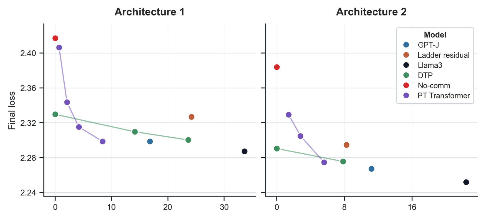
Figure 6 shows a comparison between the different state-of-the-art methods for Architecture 1 and 2 using the specificities of an AMD MI300X GPU with float8 precision. In that setup, based on our experiments, communication latency is \(\tau_c = 0.7\,\mu s\), HBM bandwidth is \(v_b = 4\,TB/s\) and precision is \(p = 1\,B\).
First, we observe that, when set in a comparable setup, DTP outperforms Ladder Residual because it reaches a better final training loss while requiring slightly less exposed wait-time.
Second, PT-Transformer has the upper-hand loss-wise when targeting roughly 5 to \(10\,\mu s\) of exposed wait-time. However, to reach lower wait-times PT-Transformer suppresses an increasing number of communications which naturally gets its performance close to the no-comm version. On the other side, DTP hides communications behind computations which allows it to reach 0 wait-time while still keeping most of the baseline performance. Hence, when targeting minimal communication overhead, DTP outperforms all presented state-of-the-art methods.
Finally, it is noticeable that as architectures grow in size and especially in hidden dimension, the domain in which DTP has the upper hand over PT-Transformer gets bigger. This is explained by the fact that the number of weights to stream by module grows with the hidden dimension, so more of the communication time can be hidden behind weight streaming. As a direct consequence, the bigger the architecture the more beneficial DTP is w.r.t PT-Transformer. With this in mind, DTP becomes the natural choice when scaling to bigger architectures.
Conclusion
In this blog post we introduced Delayed Tensor Parallelism (DTP), a new method for hiding communications behind computations in Transformer-like architectures. We showed that, compared to a no-comm version of TP, DTP was able to claw back most of the performance loss and reaches roughly the same performance as the standard TP baseline. Furthermore, we demonstrated that, in a memory-bound setup where weight streaming is the bottleneck, DTP can outperform all state-of-the-art methods for reducing communication that we are aware of, especially when targeting complete suppression of the communication overhead.
Building on these findings, we pretrained a 2B-parameter DTP model integrating Kog's inference optimizations and achieved unprecedented inference speed on AMD and NVIDIA datacenter GPUs while maintaining competitive quality loss-wise. We believe this work opens the door to a new class of latency-oriented Transformer-like architectures designed specifically for real-time, single-user inference workloads.
Future work will focus on providing a more comprehensive evaluation of DTP against existing communication-overhead reduction techniques across widely adopted benchmarks. These results will serve as the foundation for a full research paper detailing the method, theoretical analysis, and large-scale empirical evaluation.
Explore our live playground demo at playground.kog.ai and benchmark results at blog.kog.ai.
Bibliography
-
M. Shoeybi, M. Patwary, R. Puri, P. LeGresley, J. Casper, and B. Catanzaro, "Megatron-LM: Training Multi-Billion Parameter Language Models Using Model Parallelism," CoRR, 2019. [Online]. Available: https://arxiv.org/abs/1909.08053
-
S. Diao et al., "CLIMB: CLustering-based Iterative Data Mixture Bootstrapping for Language Model Pre-training," arXiv preprint, 2025. [Online]. Available: https://arxiv.org/abs/2504.13161
-
A. Chowdhery et al., "PaLM: Scaling Language Modeling with Pathways." [Online]. Available: https://arxiv.org/abs/2204.02311
-
M. Zhang et al., "Ladder-residual: parallelism-aware architecture for accelerating large model inference with communication overlapping." [Online]. Available: https://arxiv.org/abs/2501.06589
-
C. Wang et al., "Parallel Track Transformers: Enabling Fast GPU Inference with Reduced Synchronization," arXiv preprint arXiv:2602.07306, 2026. [Online]. Available: https://arxiv.org/abs/2602.07306
-
R. B. Prabhakar, H. Zhang, and D. Wentzlaff, "Kraken: Inherently Parallel Transformers For Efficient Multi-Device Inference." [Online]. Available: https://arxiv.org/abs/2408.07802