Building a single-kernel, latency-optimized LLM inference engine on AMD MI300X GPUs
We implemented the entire LLM decode pass in a single persistent kernel, no kernel launches, no interruptions, achieving 3,000+ tokens/s per request on AMD MI300X.

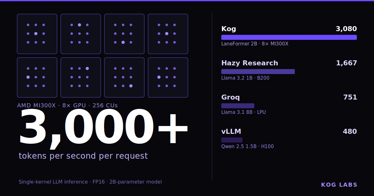
In this blog post, we present the unique challenges of serving large language models (LLMs) at low latency, and explain how the Kog AI team implemented a monokernel to achieve the fastest ever LLM decoding inference on standard datacenter GPUs (as of our knowledge at the date of this writing), generating 3,000+ output tokens/s per request for an FP16 2B-parameter model on a single 8x AMD MI300X node.
Rationale and challenges for low-latency LLM inference
LLM serving is challenging due to its broad performance requirements depending on the application type. Some, like media pipelines, batch document processing and content moderation require throughput optimized servers. Others, such as copilots, chatbots, voice assistants and interactive agents require latency optimized servers.
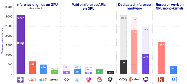
Here, we focus on latency-optimized applications. Indeed, the current inference engine implementations suffer from a sluggish execution speed for decode inference: for 2B to 8B sized models, assuming high end datacenter GPUs like NVIDIA's H100, the typical decoding speed is in the range of 100–300 output tokens/s per request. Currently, the fastest inference on programmable hardware was achieved by Cerebras, who were able to reach over 3,000 tok/s/req for GPT-OSS-120B on their custom whole-wafer chip (see Section 5 for a comprehensive discussion of other low-latency inference approaches).
Our optimized Kog Inference Engine (KIE) software achieves more than 3,000 tok/s inference speed on a single 8x MI300X GPU node, with batch size 1 in FP16 precision, on a 2B-parameter model using Delayed Tensor Parallelism (DTP). We expect to be able to extend this implementation to support higher batch sizes without significant performance loss, up to a certain point. This speed puts us well ahead of existing GPU-based implementations, and is comparable to the benchmarks measured on purpose-built hardware.
One major challenge when optimizing for inference decode latency is that commonly overlooked effects compound and become significant. To list a few, kernel launch overhead, synchronizations, workload imbalances across compute units, and tail effects can add significant overhead.
The physical limitation for the possible lowest latency on GPUs is characterized by the HBM memory bandwidth, because all model parameters need to be transferred to the compute processors in order to generate a token. This is the main bottleneck in the batch size 1 setting, where computation speed is not limited by available FLOPs. The time required for this data movement sets a lower bound on the inference latency.
Furthermore, due to the sequential nature of LLMs, synchronizations between the compute units and among the GPUs are also necessary. Synchronization time is bottlenecked by the HBM memory read and write latencies. In our case, grid synchronization is responsible for around 35% of the total token generation time.
Overcoming the challenges listed above required developing and applying several strategies:
- First, we implemented the whole sequence decoding pass in a single monokernel (including sampling). We'll explain how in the following sections of this blog post.
- Second, taking into account the hardware topology, we managed to decrease the latency of grid synchronizations. We plan to publish a dedicated blog post or paper about this (follow our blog to get notified), but meanwhile you can take a look at our talk at AMD AI DevDay 2026.
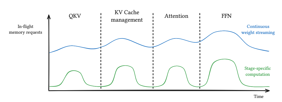
- Third, we designed a continuous weight streaming approach to load the model parameters ahead of time, avoid traffic spikes, and limit memory contentions.
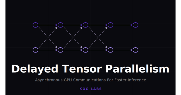
- Finally, the DTP-based Laneformer architecture was designed with delayed all-reduce communication, providing enough time to send the local outputs asynchronously and thus avoiding any additional delay due to synchronization among devices.
In this post, we focus on our monokernel implementation.
Kernel fusion and the KIE monokernel
In machine learning, model inference can be expressed as a succession of operations such as normalizations, matrix multiplications, softmax, etc. These computations are often sequential: a given operation depends on the output of the previous one. Thus, a synchronization is required between each stage, acting as both a barrier and memory coherence point. Traditionally, this is achieved by running a dedicated kernel (GPU program) for each computational step, and exploiting the consistency guarantees given by the hardware.
However, this approach has several drawbacks that can drastically limit performance, especially in a memory-bound inference setting:
- stalling all computations during each kernel launch and cleanup, an overhead that we measured experimentally to be around 4.5 µs on the AMD MI300X GPU,
- interrupting the streaming of model weights from HBM memory to the compute units for the same amount of time, while also adding a ~0.5 µs HBM latency cost when memory loads restart at the beginning of the next kernel,
- materializing intermediate tensors in the global memory of the device, which requires store/load HBM memory round-trips — usually a >1 µs overhead.
Kernel fusion has long been recognized as a high-impact optimization to alleviate these inefficiencies, by merging consecutive operations into a single GPU program. Though more powerful, it is also a much more complex approach, which is the reason why it's usually not performed, or performed automatically with higher-level abstractions, compilation, or intermediate representations and languages — at the cost of being sub-optimal.
Today, automatic (partial) fusion is an ubiquitous compilation step of modern GPU frameworks such as PyTorch or XLA.
Megakernels take fusion a step further, and unify major computational blocks of a model forward pass into a single kernel, opening unique optimization opportunities. In particular, this allows to blur the line between computational stages: the model weights for a later task can begin pre-loading while the former task is still completing, and memory streaming can continue during grid synchronizations.
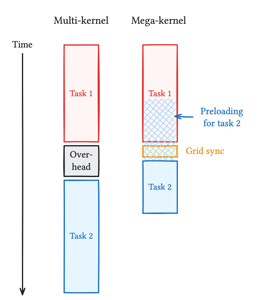
Here, we propose a single-kernel, persistent, ad-hoc implementation of LLM decoding inference, which we dub "monokernel". This approach uses programmer-managed, compile-time partition of work, thus removing the overhead of task management and scheduling sometimes found in megakernels. Every part was engineered from scratch for minimal latency, without using any third-party framework or code, and optimized specifically for the AMD MI300X.
Our monokernel processes and generates the entire token sequence (prefill and decode) until the EOS token is reached, including stochastic LM-head sampling, without any host CPU interaction. It also handles tensor parallelism requirements such as cross-device communication and reduction across lanes. It manages its own internal state, and can thus handle arbitrarily long sequences without interruption.
To our knowledge, this represents the first time the megakernel paradigm has been pushed that far for LLM inference optimization.
Implementation details
In this section, we give a brief overview of the Kog monokernel implementation. We start by detailing several patterns that are common through the whole monokernel, including innovations by the Kog team, then explain how they are used in practice within each major stage.
Programming patterns
Grid Layout
In traditional kernels, grid and block dimensions are chosen to suit the computation pattern, such as GEMMs using tile-oriented shapes. While convenient, this abstraction hides the mapping between logical blocks and physical Compute Units (CUs, equivalent to SMs in NVIDIA). In a persistent-kernel setting, one singular layout must serve all stages, so we use a hardware-shaped grid and map each stage's logical work onto it.
The MI300X features a chiplet architecture: 8 Accelerator Compute Dies (XCDs)11 The AMD MI300X features a chiplet architecture: multiple dies are assembled in a mega-chip. The compute dies, termed XCDs, contain the CUs and L2 cache. are assembled in a mega-chip. Each XCD contains its own L2 cache and 38 CUs, for a total of 304 on the entire chip. Every CU then contains 4 SIMD processors which execute work in 64-lanes wavefronts (sometimes shortened to wave, and equivalent to warp on NVIDIA).
Our monokernel uses 256 of these CUs, and launches with gridDim = (256,) and blockDim = (64, 8). This covers one wavefront in the block's x-dimension and 8 waves in the y-dimension, while the grid maps one logical block to each active CU.
We use 256 CUs because this is already sufficient to saturate peak bandwidth on the MI300X, while also maintaining compatibility with the MI355X, which has only 256 available CUs. On the other side, we choose 8 wavefronts per CU, mapping to two wavefronts per SIMD, to allow a large per-wave register allocation while still leaving enough independent waves to take advantage of hardware-enabled parallelism.
Each stage on the monokernel then decides how it should map its operation to the physical properties of the hardware.
Vector-matrix multiplication using ALU instructions
In our decode setting, all matrix multiplications are batch-1 vector-matrix multiplications: each output element is a dot product between the current activation vector and one row of the weight matrix. This is unlike the throughput-oriented regime targeted by systems such as vLLM and SGLang, where more aggressive batching results in wider GEMMs. On the MI300X, matrix-core primitives operate on matrix-matrix tiles, not native GEMV shapes, and in our case the cost of feeding those tiles outweighs the comparatively tiny amount of useful arithmetic they would perform.
We therefore choose to use scalar and vector ALU instructions, in particular dot product operations. Each CU of the GPU owns a small number of output elements, and threads load contiguous fragments of the activation vector and the corresponding packed weight rows. Because the arithmetic is expressed as regular instructions rather than as fixed matrix-core tiles, we have more freedom to place the dot2 22 The operation's internal precision is 32 bits, as operands are automatically upscaled to F32 before accumulation. operations exactly where they fit in the monokernel. Partial dot products are accumulated in FP32, reduced within the wave using Data Parallel Primitive (DPP) operations, and then reduced across waves through LDS. We encourage the reader to check our upcoming blog post on DPP cross-lanes reduction for more details.
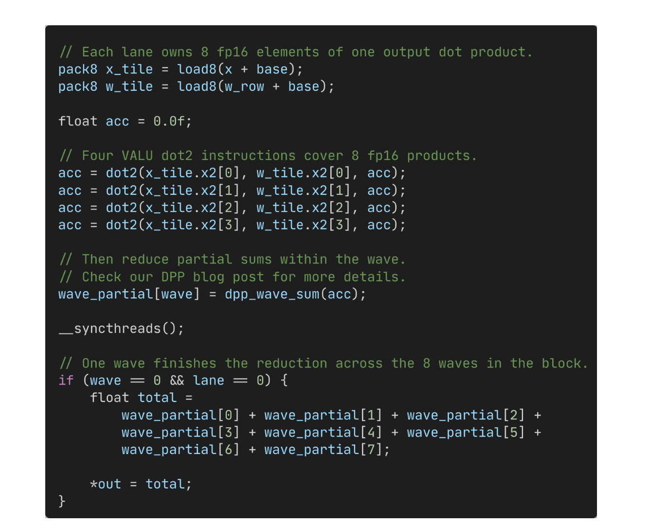
(4096,) @ (1, 4096).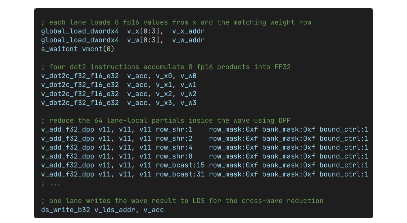
(4096,) @ (1, 4096).Fast grid synchronization primitive
Kernel cleanup at the end of each kernel execution introduces an overhead that we can avoid with a fused and persistent kernel. At the same time, kernel boundaries are exactly what makes dependencies between computational sections easy to manage: once the next kernel starts, the previous phase is finished by design. In a monokernel we lose that convenience, so synchronization and acquire-release semantics must be managed explicitly inside one resident program.
A traditional software approach is arrival counters plus epochs. Each CU first synchronizes its local waves (easily done with __syncthreads()), then a designated thread atomically increments a global counter. When the counter reaches the number of participating CUs (typically 256), one CU advances an epoch, and the rest spin-wait until they observe the epoch change. In practice, this scheme is paired with operations such as __threadfence() so producer stores are visible before consumers proceed.
This is robust, but expensive for latency-oriented decode. Per sync point, a CU pays at least one global write (counter arrival), one global read path (epoch polling), while the final arriving CU additionally pays one more global write to advance the epoch, as well as ordering/cache-management overhead before it can safely consume payload data. Operations like __threadfence() can lower to buffer_wbl2 + buffer_inv instructions, that write back dirty L2 cache lines to HBM and invalidate L1/L2 cache lines, respectively.33 Exact behavior depends on cache policy bits. This means that even when the next stage needs only a small subset of values, the system will force broad cache movement and extra HBM traffic. Moreover, atomic contention on the shared arrival counter can further increase barrier latency due to serialized reads.
We wanted a different approach: lighter synchronization semantics, where consumers wait only on the values they actually need, and no unrelated HBM round-trips in this latency-critical path.
But can it be achieved? Yes, by rethinking the synchronization design.
Our core idea is to encode readiness in the data path itself. Publish-dependent buffers are initialized to a sentinel value (e.g. NaN), and consumers poll those same locations until the sentinel disappears, which indicates that real data has been published. There are two caveats that needs to be managed carefully for this approach to work:
- First, the sentinel region must be reset before reuse. We avoid overheads associated to these buffer resets by using multiple buffers and asynchronous resets.
- Also, the sentinel value must be outside the set of valid outputs. Fortunately the floating point standards provide multiple avenues for sentinel values, the most obvious being
NaNwhich should never appear in an LLM activation vector.
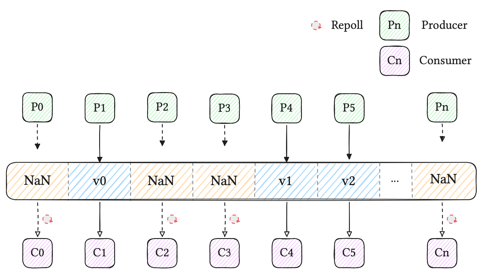
Additionally, for correctness, reads and writes on these handoff locations must use the intended scope-control semantics (for example global_load/global_store ... sc1 at device scope). This guarantees that read-write operations will skip the non-coherent L1, and use the scoped L2 coherence behavior required for correct cross-chiplet communication on the MI300X.
This gives us a synchronization point tied directly to the actual data dependencies for each CU, instead of a broad grid-wide phase barrier, and our results reflect that:
| Method | Latency Range |
|---|---|
| Kog | 0.80–0.93 μs |
| Naive | 7.59–7.88 μs |
This synchronization pattern appears throughout the monokernel, and is further strengthened by exploiting program order (as we will see in Section 3.2.1), physical topology of the GPU (as we will see in Section 3.1.6), and a few other innovations proprietary to Kog.
Continuous weight streaming to LDS and registers
A crucial advantage of monokernels is the ability to prefetch weights across inference stages. Since the same program is executing the entire computational sequence, we can overlap memory accesses with prior compute or synchronization operations. In short, monokernels allow for extremely deep pipelining.
We use two kinds of loading instructions: to local memory and to registers. Loads to local memory (i.e. LDS on AMD GPUs) allow for maximal flexibility, since all threads of a block have direct access to it. They also bypass the register file, which decreases register pressure. However, the LDS on the MI300X has a relatively small capacity (64 KiB), so not all weights can be prefetched this way. For the remaining data, we use standard loads to registers.
In addition, all weight loading operations are done with non-temporal (streaming) requests by using NT scope bit on the load instructions. This hints the cache subsystems to deprioritize storing weights, and alleviates cache pressure for other useful data.
Offline preprocessing
Because the kernel is severely memory bound, we try to remove avoidable runtime memory traffic and make the remaining memory accesses as regular as possible, using existing (and some new) ideas.
One common offline weight transformation is RMSNorm folding. Many projections are preceded by RMSNorm, whose scale vector is static. It's possible to fold this scale directly into the projection weights during model conversion. At runtime, the kernel only computes the dynamic RMS factor, avoiding a separate load of hidden_size normalization weights.
The same idea applies to the weight layout. Because the monokernel has a fixed execution schedule, we know ahead of time which rows each CU will consume and in what order. This means the tensor layout does not have to match the framework layout used during training or export. If another layout better matches the runtime access pattern, we can store the weights in that layout before inference starts.
The QKV projection is the clearest example of this. A standard layout would store Q, K, and V as three separate contiguous matrices. However, the kernel consumes their rows in interleaved groups, we therefore repack those rows offline in exactly that execution order. When the kernel runs, each CU can stream its assigned rows with coalesced accesses and no runtime indirection.
Another form of preprocessing is the preparation of static runtime tables. Although this is not primarily a memory-bandwidth optimization, it still removes work from the runtime path when the values are fully determined ahead of time. For RoPE, we precompute the rotary values offline up to the maximum supported sequence length, storing them directly in the format expected by the kernel.
Topology-aware memory accesses
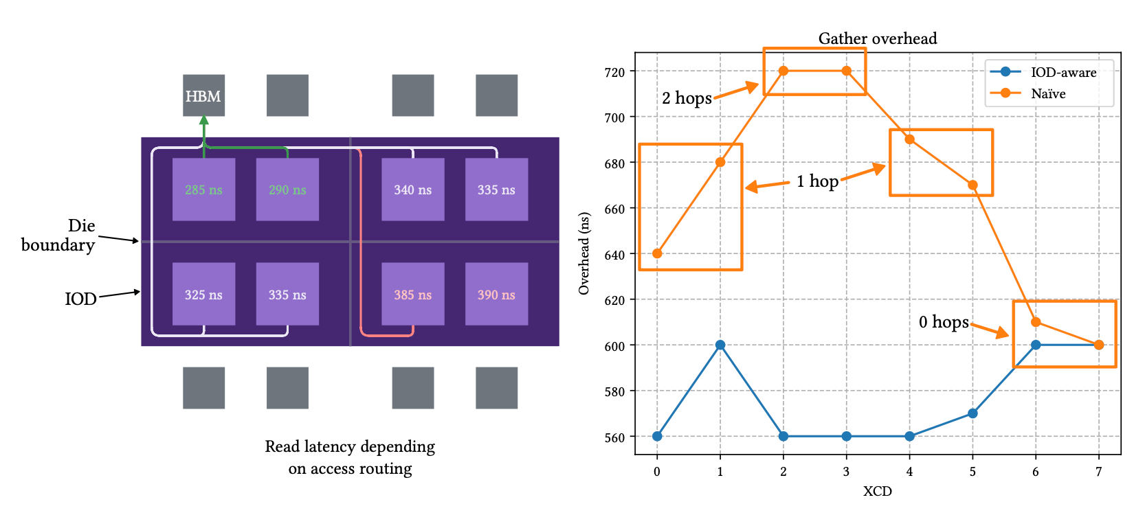
During device-scoped reduction operations, the CUs must communicate through global memory. Due to the hardware organization of the MI300X, in particular the I/O die layout, this can incur an asymmetric latency for some CU, because of the additional hops across die boundaries.
In order to mitigate this, we employ a IOD-aware strategy: the tensors are duplicated per I/O die, and the CUs then read them from their own attached die. This process required reverse-engineering the mapping function from physical addresses to IOD location, and designing an algorithm to recover the physical address of a device memory allocation, which will both be expanded upon in a future Kog Labs blog post.
With this strategy, the synchronization overhead is flattened to the best-case scenario for all CUs, where no cross-die connections are taken.
Per-stage details
The first model we support in our monokernel is a Laneformer architecture, a variant of the Transformer architecture designed and trained by the Kog team, for a 2B-parameters model parallelized in 8 "lanes" distributed on the 8 GPUs of a node. That being said, the following concepts apply to any standard Transformer architecture as well.
QKV projection
Each Laneformer lane uses 4 Q heads, 2 K heads, and 2 V heads, all with head dimension 96. The QKV projection therefore produces a total of 768 scalar outputs per lane. With 256 active CUs, we map this to three scalar outputs per CU, where each scalar is the result of one GEMV, computed as a dot product between the normalized activation vector and one row of the packed QKV projection weights.
These values must then be handed off to attention. Attention needs every query on every wave, so Q values must be gathered using the polling-based synchronization mechanism described above. In principle, K and V values also need the same treatment: they are produced by the QKV stage and consumed by attention, so consumers must not read them before they have been published.
However, because every wave already polls all Q values, this opens a useful opportunity: if a CU publishes its K/V values before publishing a Q value, and those stores are issued by the same thread, then observing that Q value also guarantees that the earlier K/V stores from that CU have completed, because vector memory operations of the same type retire in program order on CDNA3 (see section 4.4 of the CDNA 3 ISA reference).
Therefore the current-token K and V never become synchronization targets themselves, the Q-polling serves as the readiness signal. The decoupling from a separate current-token KV polling path allows the entire KV cache to be read as a consumption stream with minimal control flow, allowing the agent-scoped loads to be flexibly scheduled and waited on only when attention actually consumes them. In our implementation, this completely hides the V-loading path.
This requires every CU to produce at least one Q scalar among its three outputs. We therefore choose an interleaved QKV row mapping with that constraint, and repack the projection weights offline to match it. This keeps the QKV handoff aligned with the attention-side streaming schedule, reducing total handoff time.
Attention
The attention in Laneformer has both a sliding window attention and a full-context causal attention. The latter can take into account the whole sequence history through the KV cache. Our implementation therefore adapts a general approach.
The attention formula is \(A = \text{softmax}(QK^T)V\), then \(y = W_o A\) where \(W_o\) is the output projection matrix.
- \(Q\) has a shape of:
(num_attention_heads, head_dim) - \(K\) has a shape of:
(seq_len, head_dim * num_kv_heads) - \(V\) has a shape of:
(seq_len, head_dim * num_kv_heads) - Output shape:
(num_attention_heads, head_dim)
The best way to split the workload among the CUs is along the sequence length dimension. This prevents the manifestation of long columns from \(K\) and \(V\) in each CU. But this comes with the cost of aggregating the partial results calculated by the CUs. In our implementation the attention block has three main stages:
- per-CU attention
- cross-CU aggregation
- output projection.
The per-CU attention implements the \(\text{softmax}(QK^T)V\) attention in each CU independently. Each CU is responsible to apply the attention on a small tile of the KV cache. This stage applies the softmax for the sub-tiles, meaning the reductions necessary for the softmax calculation does not span over the whole sequence of \(K\). These local results later requires correction to get the right softmax values in each sub-tile.
In the aggregation stage, the results in each CU are corrected after the tile level softmax data is shared. A sum-reduce over the corrected sub-tiles finalizes the matrix multiplication by \(V\). At the end this results in a small, flat vector with 384 elements.
Finally, the third stage calculates the output projection. Here, each CU divides the workload by calculating the matrix-vector multiplication on a subset of rows of the \(W_o\) matrix.
Each stage is separated with grid synchronizations. The two grid synchronizations are necessary to share the temporary results after the first and second stages. To make the attention implementation more chiplet-aware, the first and second stages use recomputation. The AMD MI300X card has 4 IODs, each connected to 2 HBM stacks and 2 XCDs (see Section 3.1.6). To avoid the cross-IOD communication-related penalty during the grid synchronizations, 64 CUs on each IOD forms a group and calculate the first and second stages independently. Therefore at the end of the second stage, four copies of the same output will be available. The effect of recomputation is increased computational and memory load per CU, but less data exchange during synchronization.
FFN
We exploit weight streaming in particular for the feed-forward network (FFN) stage of decoder layers. For dense models, this represents by far the most memory-intensive task of the inference process: in the Laneformer model, almost 80% of layer weights are dedicated to FFN stages.
Model weights are prefetched during the attention stage, in particular during its compute-intensive tasks and while doing synchronization work. The entirety of the W1/W3 tensors are pre-loaded before entering the FFN section. W2 is loaded partly during attention, with the remainder fetched during the FFN internal projection.
Delayed Tensor Parallelism (DTP)
Delayed Tensor Parallelism is a key innovation of the Laneformer LLM architecture. TP reductions from the attention and FFN stages are delayed by associating them with subsequent layers. This enables fully asynchronous cross-device communication and hides Infinity Fabric (xGMI) latency behind the processing of other layers. The overhead of TP is thus reduced to near-zero, with only the cost of the 8-way reduction partially remaining.
Language-modeling head
The LM-head does a global reduction across all devices to select the next token from a probability distribution over vocabulary space.
We first perturb the logits with Gumbel noise, then select \(\text{argmax}(\text{logits} + \text{Gumbel})\) as the predicted token. This construct is equivalent to the usual softmax version, but allows the global reduction to be a simple argmax without needing to share the full probability tensor. Thus, the CU can share partially reduced results instead of the whole distribution, which greatly cuts the cross-device traffic (in our case, we decrease it by close to 800%).
Writing a monokernel, in practice
Compiler limitations
The complexity of our monokernel also posed challenges for the compiler. The difficulty arose mainly from the presence of inline assembly and the limited number of registers.
We typically used inline assembly when an instruction was not possible to apply with any built-ins. For instance, __hip_atomic_load and __hip_atomic_store were important for us during synchronization. But these functions can not support a data type of 3 dwords. We had to use an inline assembly to insert a global_load_dwordx3 with the sc1 bit enabled. The compiler is not able to track dependencies for such operations (even with a memory clobber modifier), so we had to manually insert the required s_waitcnt instruction for correct ordering.
Speaking of s_waitcnt, the compiler can add s_waitcnt vmcnt(0) instructions (as shown in Figure 2) which will stop memory streaming. We had to be mindful of this and manually tweak the code to control the locations of such wait instructions.
Our source code for the decoder layer uses a lot of address calculations. The decode inference requires two big outer loops, one for executing the decoder layer multiple times and one for calculating the tokens. Loop Invariant Code Motion (LICM) is a technique used by the compiler to move some calculations outside of the loop and save their results in registers. Address calculations can have several parts not depending on the layer index, therefore they can be calculated only once before entering the loop. This increases register pressure.
So we had to be very careful to avoid register spills which generally have a detrimental impact on performance. Deep inspection of compiler output, and better algorithmic choice at the micro level helped to eliminate these situations.
We carefully inspected every assembly instruction emitted by the compiler and made the necessary adjustments to ensure optimality and adherence to our intentions. We found that Compiler Explorer is quite useful for quick checks and sharing results across the team.
Team collaboration
Writing a monokernel requires careful coordination. Unlike conventional implementations, where stages live in separate kernels, many stages here share the same launch configuration, synchronization mechanisms, buffers, register budget, and LDS usage. As a result, local changes can affect unrelated parts of the model through timing changes, CU or wave misalignment, or resource pressure.
To make this workable, we used explicit stage ownership. Each person owned a major stage, such as QKV, attention, or FFN, implemented behind an inline function with a narrow interface. Whole-kernel mechanisms followed the same idea: cross-stage reductions, buffer lifetime management, layer handoff, and full-loop integration usually had a single owner across all stages.
The same applied to debugging: because bugs in a monokernel are often non-local, debugging also required coordination across the whole team. We relied on reference implementations and regular testing. During our first full integration pass, leaking NaN values forced everyone to audit the whole codebase, not only their own stage. This was slow, but gave the team a much better understanding of interactions between stages, synchronization, buffers, and control flow.
In practice, our collaboration model followed three principles: give each major stage a clear owner, keep common control-flow areas small, and regularly audit the whole monokernel as a team.
Profiling
Reaching extreme performance levels is not possible in a vacuum, and requires advanced tooling to identify, understand and fix bottlenecks.
Commonly, profiling tools such as rocprof are used to collect performance counters, and perform instruction-level tracing. In a megakernel context, the amount of data collected can quickly become intractable (if the tools can even handle it). In addition, it can be tricky to disentangle metrics from different computational stages, since tools often do not offer the possibility to perform fine-grained analysis.
We have addressed these issues with a 3-folded approach:
- standalone kernels: we can produce programs for individual stages (e.g. attention, FFN), or higher-level primitives (e.g. decoder), that can be profiled with the aforementioned tools (in particular, rocprof-compute for counter collection, and rocprofv3 for tracing in conjunction with rocprof-compute-viewer for visualization).
- dynamic counter collection: we exploit the hardware's ability to dynamically enable counter collection (for e.g. in-flight memory instructions, hardware stalls, etc). Thus, we can focus on arbitrary parts of the monokernel, without polluting the metrics with unrelated code.
// Dynamically enable perfcounting for a particular CU using the MODE.DISABLE_PERF special register field
__device__ __forceinline__
void disable_perf_counting() {
    __builtin_amdgcn_s_setreg(0x0681, 1);
}

__device__ __forceinline__
void enable_perf_counting() {
    __builtin_amdgcn_s_setreg(0x0681, 0);
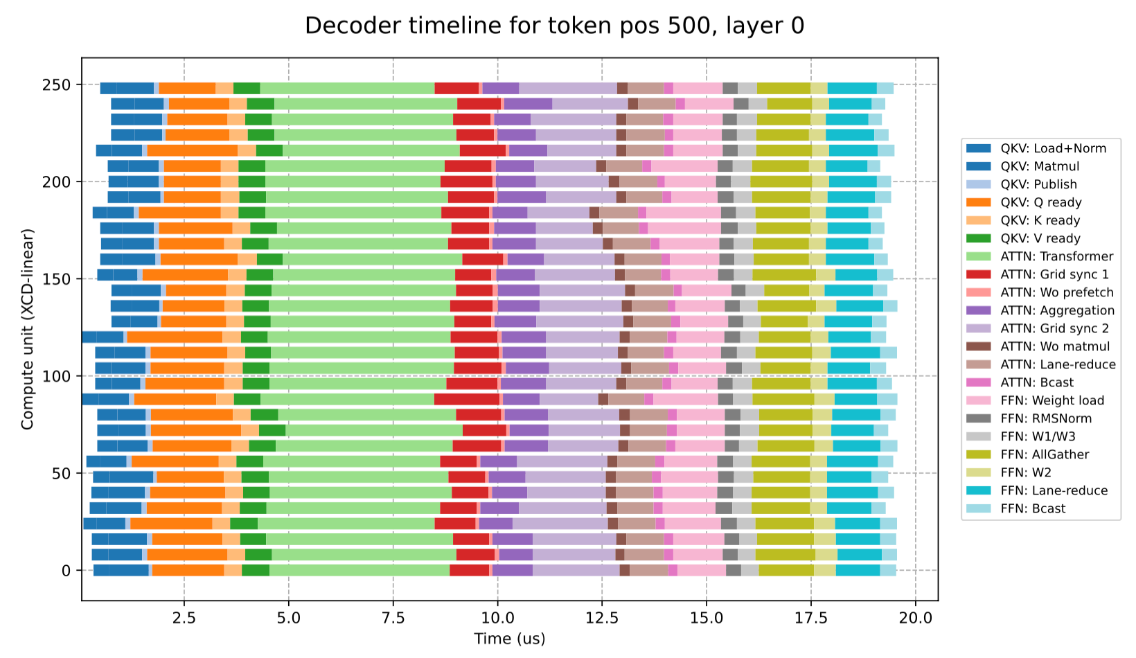
}- custom benchmarking framework: the monokernel can be compiled to an instrumented version, that will collect device timestamps. We convert these timestamps into a common system-clock domain using HSA API functions, this gives all 8 GPUs a shared time reference and makes it possible to profile cross-GPU communication directly. The data can then be analyzed to produce a timeline and/or statistics on runtime behavior, such as the picture below (which represents a trace over a model layer for a single CU).
The combination of these tools enables powerful performance analysis at any depth level.
Prior art in low-latency LLM inference decoding
Several techniques and approaches have been developed to implement low-latency LLM inference, ranging from creative GPU programming patterns, to dedicated hardware. We'll briefly cover two of them: megakernels and hardware designs.
Megakernels
Broadly speaking, two megakernel techniques exist: ad-hoc implementations and on-device interpreters.
While we exposed the many advantages of megakernels in previous sections, their drawback is mainly the lack of scalability in development. Several projects try to address this with compilers which automate the generation of such programs.
Hardcoded megakernels
This method is conceptually simple, but perhaps more tricky to implement: essentially, it entails creating a single program that handles multiple stages of computation with hard-coded control flow. This requires careful workload partitioning, since the launch configuration is fixed across the whole program and computation routinely uses different shapes. Failing that, it can easily lead to hardware under-utilization or poor memory access patterns. Prior work includes several mega-kernel implementations of the entire forward decode pass for the Qwen family of models. On Qwen 3 0.6B, upwards of 1000 tok/s have been reported on a single NVIDIA 5090. Moreover, fused kernels for critical and complex tasks such as MoE and MLA have also been proposed.
Frameworks and Runtimes
Between fully hand-written and compiler-generated fused kernels, there is a middle layer of frameworks and runtimes that still require explicit GPU programming, but provide an abstraction over low-level mechanisms in order to facilitate development. These systems do not remove the need to reason about the hardware. Instead, they give programmers a more structured vocabulary for expressing patterns that otherwise become ad-hoc control flow, such as tiled data movement, memory consistency and synchronization.
Hazy Research's megakernel work is an example of this middle layer on NVIDIA GPUs. ThunderKittens44 A version focused on AMD hardware has been released since then. is a CUDA-embedded framework built around tile abstractions, managed layouts, and producer/consumer templates for asynchronous work. Their Llama megakernel, which reaches around 1500 tok/s on B200, adds an on-GPU interpreter, where each Streaming Multiprocessor (SM) executes a statically planned sequence of coarse-grained instructions55 These are not bytecode-style scalar instructions; they are logical model operations, such as attention or the LM head. defined by the kernel author. Additionally, shared memory paging allows the interpreter to know how much and which places of shared memory are available, enabling weight streaming, one of the major advantages of persistent kernels. These abstractions make a whole-model megakernel programmable without writing monolithic control flow by hand. However, the runtime also must still explicitly manage inter-instruction dependencies through global-memory counters.
Fleet takes a different route and is especially relevant to our setting. Developed by AMD, it is a hierarchical task model and persistent-kernel runtime explicitly aimed at megakernels on multi-die GPUs. The persistent kernel is composed of multiple workers and one scheduler per chiplet. Tasks dispatched to the scheduler are classified at different levels of the hardware hierarchy, so that each task runs at the narrowest sufficient scope: wavefront, CU, chiplet/XCD, or device.
This hierarchy directly ties scheduling decisions to memory consistency and synchronization, as the level at which a task runs determines the level at which its dependencies must be made visible. Fleet therefore encourages the programmer to express the smallest scope at which a task can run correctly, making synchronization a local operation whenever the dependency structure allows it.
This is most apparent in the distinction between chiplet-level and device-level tasks. A chiplet-task binds work and data to a single XCD, and coordinates CD's local L2 cache, avoiding coherent traffic across the cross-chiplet fabric. Device-level tasks, on the other hand, are used when dependencies must cross chiplet boundaries. In that case, Fleet escalates to global synchronization, but avoids making every worker pay the full cost by having only the last worker on each compute die (XCD) issue the required fence and update the global event counter.
Still, this two-fold approach pays the price of increasing and polling counters in the L2-cache, as well as a full threadfence(), which again can lower to buffer_inv and buffer_wbl2, resulting in broad data movement from the L2-cache. This underperforms our fine-grained grid synchronization method that completely avoids operating over any memory except the to-be-shared data.
Finally, it is important to note that Fleet's scheduler operates only at the intra-GPU level.
Compilers
Compiler-based megakernels aim to get the latency benefits of monolithic GPU programs without writing every model implementation by hand. They start from a high-level model or tensor program, then automatically fuse, schedule and lower it into a persistent kernel that removes launch overhead, reduces intermediate memory traffic, and overlaps independent work.
Luminal frames this as ahead-of-time inference compilation: the model is lowered to a graph IR, optimized through fusion, tiling, memory planning and scheduling, then emitted as native GPU or ASIC code. Its megakernel direction is motivated by three concrete decode bottlenecks: kernel launch overhead, uneven SM utilization from wave quantization, and idle compute during weight loading.
Mirage Persistent Kernel takes a more explicit compiler and runtime system approach. It lowers tensor programs into SM-level task graphs, where dependencies are represented at the granularity of individual SMs, and an in-kernel decentralized runtime schedules those tasks inside one persistent megakernel. This enables cross-operator pipelining and fine-grained overlap across computation and communication.
The common idea is to compile the model inference logic into one globally scheduled GPU program: operators are fused, task scheduling is done on the device, and independent work can overlap inside a persistent kernel.
Drawbacks of these compilers include:
- overheads introduced by generic runtimes, conservative code generation, and non-zero-cost abstractions,
- reduced low-level control,
- as a consequence, hardware- or model-specific tricks can be missed, while a hand-written monokernel can research and exploit them.
Specialized hardware
Beside GPUs, new hardware vendors are trying to provide novel approaches to achieve better inference performance for LLMs. Here are some examples, with a quick summary of their design choices and trade-offs.
Cerebras' Wafer-Scale-Engine (WSE) was reported to achieve 3,000 tok/s on GPT-OSS-120B (5.1B active parameters) model. The WSE uses only on-chip SRAM, no DRAM, providing 21 PB/s memory bandwidth, compared to the 4.3 TB/s HBM empirical memory bandwidth on one MI300X GPU and 34.4 TB/s on a full 8x MI300X node. In a memory-bound workload, this removes the memory bottleneck which is incredibly beneficial. However it should be noted that other bottlenecks exist, for instance communication and grid synchronization speed between all processors on the wafer. Also, a WSE has only 44 GB memory (compared to 192 GB on a single MI300X GPU and 1.5 TB on a full node), which means models with more parameters either need to be aggressively quantized, causing accuracy loss, or use sequential model pipelining on several chips. The latter results in chip-to-chip network communication at higher latency and lower bandwidth than intra-node GPU-GPU communication.
Groq's LPU (language processing unit) also targets fast AI inference. Their approach has four principles: software first, programmable assembly line architecture, deterministic compute and on-chip memory. The programmable assembly line makes possible to avoid waiting for compute and memory resources to compute a task. On-chip SRAM memory provides high bandwidth. The LPU based systems can achieve up to 500 tok/s on GPT-OSS-120B. The limited amount of on-chip SRAM memory means serving a 70B model smoothly requires hundreds of LPUs, creating substantial capital requirements.
SambaNova's RDU (reconfigurable dataflow unit) is designed to efficiently move data among compute units. The dataflow is enabled through a grid of Programmable Compute Units (PCUs) and SRAM Programmable memory Units (PMUs). The data is rooted by the switching fabric. One notable difference to pure SRAM-based systems is SambaNova's three-tier memory architecture (DDR DRAM, HBM, SRAM). This makes possible to run large models with several trillion parameters and with large context windows, it also enables fast model switching for agentic workflows. The RDU based systems can achieve 700 tok/s on GPT-OSS-120B and around 270 tok/s on DeepSeek R1 0528 FP8.
Taalas' HC1 prototype promises 17000 tok/sec on LLama-3.1 8B. It's a fixed-function hardware that essentially hardcodes the specific model architecture in silicon, while other solutions retain programmability. For now, they need 3-bit and 6-bit precision, hence experiencing significant accuracy loss.
Conclusion
In this blog post, we showed the path to low-latency LLM inference on GPUs, and featured our own monokernel achieving 3,000 output tokens/s per request on AMD MI300X, powered in part by an unprecedented level of kernel fusion. Among other things, this approach eliminates multiple sources of overhead, and allows maximal flexibility in weight streaming.
It should be noted that, while we focused this post on our AMD GPU techniques, we also built a similar monokernel for NVIDIA GPUs. It currently generates 2,100 output tokens/s per request on a single 8x H200 node, with more optimizations coming.
A huge thank you for reading us! Consider following Kog Labs blog for upcoming write-ups on our other GPU optimization research results.